Introduction

Last month, I spoke with Sanyam Bhutani and demoed Gretel’s SDK with the developer community from WandB. You can watch the full workshop here. 

In preparation for the event, I had fun experimenting with some of Gretel’s projects using Weights & Biases machine learning tools, specifically their hyperparameter sweeps and visualizations. Below is an example of how you can use their tools to help optimize a synthetic model for a challenging dataset. If you’d like to follow along you can use this example notebook.

Sweeps: The Basics  🧹🧹🧹

Before we dive in, a quick primer on why you need hyperparameter sweeps. Before building any ML model, you want to determine the best variables to use with your learning algorithm, as these determine the model’s structure (e.g. the number of hidden units) and how the model is trained (e.g., learning rate, optimizer type, batch size). These are the knobs that we can control in the machine learning process.

The rub is that testing for these ideal training values manually gets unwieldy fast. That’s where MLOps tools like Weights and Biases can help. Essentially, WandB automatically “sweeps” through hundreds of combinations of hyperparameter values to find the best ones. Once finished, it provides a rich set of visualizations to inform your training process. 

With that background, let’s test the sweeps and create some synthetic time-series data!

Optimizing our synthetic model hyperparameters

For this example, we will use Weights and Biases’ tools to run a series of hyperparameter sweeps to optimize our model’s training to generate the highest quality synthetic data possible. Follow along with the end-to-end example in this Colab notebook! 

First, according to Weights and Biases documentation, you define the sweep by creating a dictionary or a YAML file that specifies the parameters to search through, the search strategy, the optimization metric et al. There are a few search methods to choose from – grid Search, random Search, or bayesian Search – each has pros and cons, depending on the project you’re tackling. We’ll stick with a bayesian Search for this example:

sweep_config = {
   'method': 'bayes'
   }

For bayesian sweeps, you also need to tell us a bit about your metric. We need to know its name, so we can find it in the model outputs and we need to know whether your goal is to minimize it (e.g. if it's the squared error) or to maximize it (e.g. if it's the accuracy).

metric = {
   'name': 'sqs',
   'goal': 'maximize'  
   }
 
sweep_config['metric'] = metric

If you're not running a bayesian Sweep, you don't have to, but it's not a bad idea to include this in your sweep_config anyway, in case you change your mind later. It's also good reproducibility practice to keep note of things like this, in case you, or someone else, come back to your Sweep in 6 months or 6 years and don't know whether val_G_batch is supposed to be high or low.

Next, you’ll define your hyperparameters:

parameters_dict = {
    'epochs': {
        'values': [25, 50, 100, 150]
        },
    'learning_rate': {
        'values': [0.001, 0.005, 0.01]
        },
    'vocab_size': {
          'values': [0, 500, 1000, 10000, 20000]
        },
    'rnn_units': {
          'values': [64, 256, 1024]
        },
    'batch_size': {
          'values': [64, 256]
        }
    }

sweep_config['parameters'] = parameters_dict

Once that’s done, you’ll initialize the sweep with one line of code and pass in the dictionary of sweep configurations: sweep_id = wandb.sweep(sweep_config)

Finally, you’ll run the sweep agent, which can also be accomplished with one line of code by calling wandb.agent() and passing the sweep_id to run, along with a function that defines your model architecture and trains it: wandb.agent(sweep_id, function=train). And you’re done! 

While there’s a lot going on under the hood, the output is a series of detailed data visuals that tell you everything you need to know – we’ll highlight two of them: 

The Parallel Coordinates Plot‍

According to WandB, this plot maps hyperparameter values to model metrics. It’s useful for honing in on combinations of hyperparameters that led to the best model performance. As you can see, using a smaller number of RNN units (256), and character-based tokenization (by using a vocab_size of 0, versus sentence piece for higher) yielded the optimal Synthetic Quality Score. This is most likely due to the relatively small amount of data, where a more complex neural network or vocabulary was not required.

The Hyperparameter Importance Plot‍

This plot surfaces which hyperparameters were the best predictors of your metrics. So depending on the metric we want to focus on (e.g., epoch, accuracy, loss, training time), we get some detailed analysis. For example, here are our best predictors with respect to accuracy:

Train your model, sample the final dataset & compare the accuracy

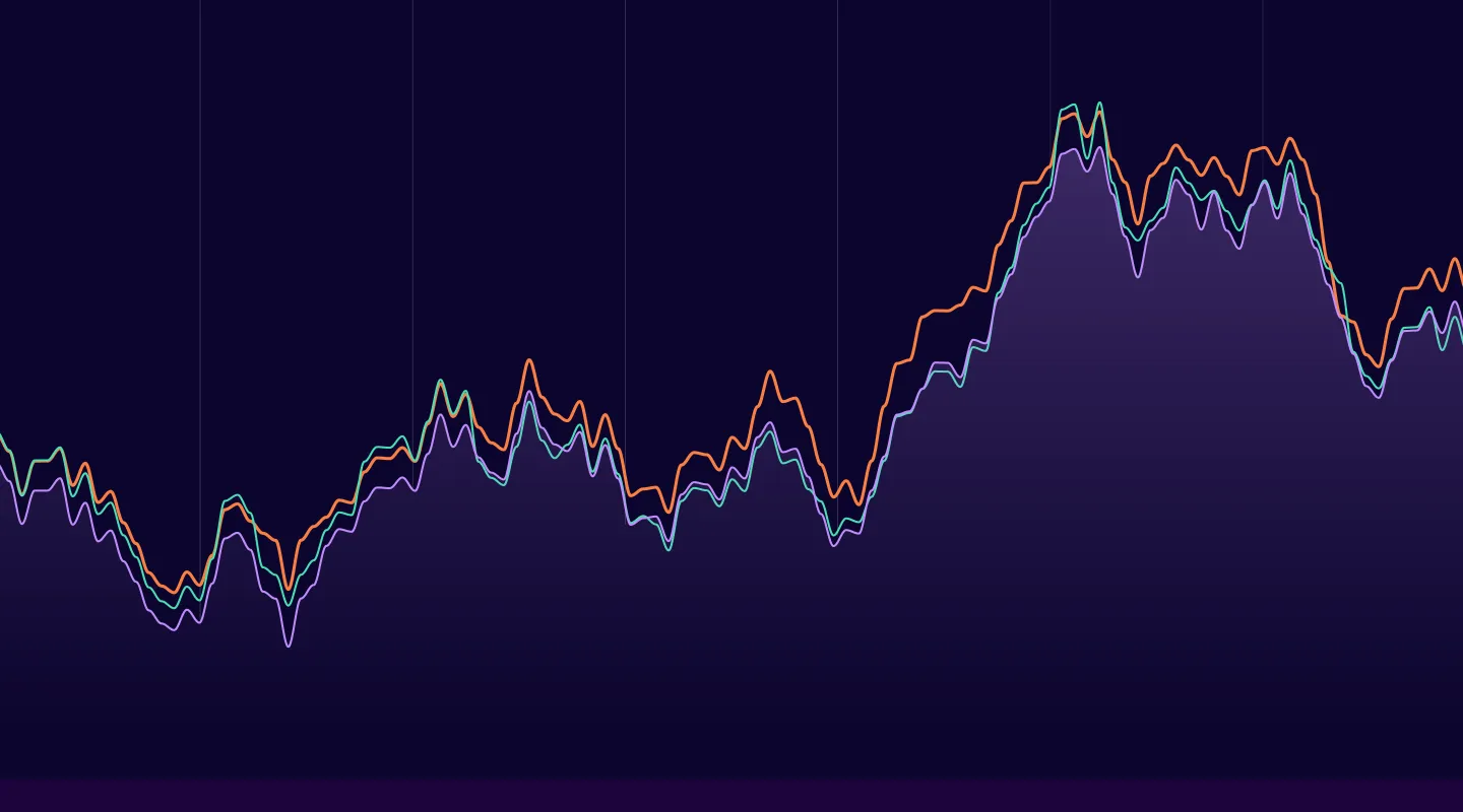
Finally, now that we’ve trained a synthetic model with optimized hyperparameters (thanks, WandB!), we can now use the optimal configuration to generate a synthetic dataset for the ML task.

Based on these charts, we can see that our model tracked closely with the real-world dataset and the synthetic data output is a quality replica of the original model.

But before we celebrate, we want to make sure that no real-world data was duplicated i.e., no personally identifiable information was ingested or replayed by our synthetic model. Gretel’s Synthetic Data Report provides some nice summary statistics to answer these questions. It includes an analysis of the field correlation and distribution stability, as well as the overall deep structure of our model.

The report provides more granular analysis, too, including mappings of correlations that exist between your training and synthetic datasets, and principal component analysis of the individual distributions of elements within those datasets. 

Conclusion

It’s exciting to see how other open-source dev tools, like Weights and Biases, can be integrated into the Gretel synthetic data generation process. If you like the WandB visualizations, you should definitely run Gretel’s colab notebook yourself, as well as watch the workshop video. 

If you’re new to Gretel, you can sign up to our free tier and run our APIs to Synthesize, Transform, or Classify data – no code required! As always, we’d love to hear from you, either by email at hi@gretel.ai or on our community Slack. Thanks for reading!