The Gretel Console provides several views and tools to help explore your data.  Another option that may work well with common existing workflows is to load the data into Elasticsearch and use Kibana for exploration and reporting.

This blog post walks through the structure of Gretel records, including NER results, and shows a simple workflow for loading that data into an Elasticsearch cluster

Getting the Blueprint

The blueprint accompanying this blog post uses docker to stand up a local Elasticsearch instance.  For this reason we recommend downloading the blueprint and running it locally.  To do this, first check out the Gretel Blueprints repository.  Using the command line and assuming you have git and jupyter-notebook installed, here is one way to do it:

cd /tmp && git clone https://github.com/gretelai/gretel-blueprints.git
cd gretel-blueprints && jupyter-notebook

You can now navigate to the blueprint in a browser.  The very last cell of the blueprint will delete our project and shut down the docker containers.  If you are going through the blueprint and this blog at the same time, or if you want to interact with Kibana before tearing everything down, please run one cell at a time.

You will also need your API Key to complete the blueprint.  You can find it in the Gretel Console at https://console.gretel.cloud/users/me/key.

Running Elasticsearch, beyond the blog

As mentioned above, in this blueprint we use docker to start up a local Elasticsearch cluster.  The docker-compose.yaml in this directory was gratefully borrowed from How to run an Elasticsearch 7 single node cluster for local development using Docker Compose?

Another option is to install the necessary Elasticsearch packages directly using a package manager such as Homebrew or yum.  Elasticsearch is also available as a managed service offered by cloud providers if you want to set up a production service.  Using a cloud hosted Elasticsearch cluster may affect how you create the Elasticsearch client in code.  It may also give you other options for writing the data to the cluster (AWS Kinesis Firehose, for example).  The code for creating a Gretel client and using it to pull records would still be mostly the same (but see comments about "forward" and "backward" directions below).

Bootstrapping a project with sample data

Gretel makes a few different sample data sets available.  We access one of these, a set of bike order data, using the Gretel python client and use this to create a new project.  We can then pull back a record from this new project to show its structure and highlight different features.  To do this, insert a cell in the notebook below the one where we call project.send_bulk.  Add the following code to the cell and try running it.  You should see a Gretel record in all its glory.

import json

records = project.iter_records(
        # NOTE that default direction is "forward".
        # In forward mode, client will block and wait for new records.
        direction="backward",
        record_limit=1, 
        params={"flatten": "no"})

for record in records:
    print(json.dumps(record, indent=4))

Structure of a Gretel Record

The first thing to note is that the original record is retained and available under the "record" key.  By default, the record will be flattened; however, Elasticsearch will reject key names with periods in them.  In the notebook we use the params={"flatten": "no"} kwarg to preserve nesting in the record.  The original record embedded in the Gretel record will look something like this:

{
    "record": {
        "CustomerID": 27390,
        "Title": null,
        "FirstName": "Leah",
        "MiddleName": null,
        "LastName": "Zeng",
        "Suffix": null,
        "AddressLine1": "9255 Katharyn Drive",
        "AddressLine2": null,
        "City": "Burien",
        "StateProvinceName": "Washington",
        "CountryRegionName": "United States",
        "PostalCode": "98168",
        "PhoneNumber": "543-555-0158",
        "BirthDate": "1940-07-13",
        "Education": "Graduate Degree",
        "Occupation": "Management",
        "Gender": "F",
        "MaritalStatus": "S",
        "HomeOwnerFlag": 0,
        "NumberCarsOwned": 2,
        "NumberChildrenAtHome": 0,
        "TotalChildren": 3,
        "YearlyIncome": 95581
    }
}

Record Metadata

Gretel writes NER findings to the metadata section, organized both by field and by entity. In the fields section, each field has a list of matching labels. Within each label object the label is the entity type. Other fields in the object give more details about the matching snippet.

"metadata": {
        "gretel_id": "ca5303e8e64b4551832519d3032e3d81",
        "fields": {
            "PhoneNumber": {
                "ner": {
                    "labels": [
                        {
                            "start": 0,
                            "end": 12,
                            "label": "phone_number",
                            "score": 0.8,
                            "source": "regex_us_phone",
                            "text": "543-555-0158"
                        }
                    ]
                }
            },
            "PostalCode": {
                "ner": {
                    "labels": [
                        {
                            "start": 0,
                            "end": 5,
                            "label": "us_zip_code",
                            "score": 0.8,
                            "source": "regex_us_zipcode",
                            "text": "98168"
                        }
                    ]
                }
            }
        },

Under the entities key, the detected entities are first organized by high/med/low score. Following this are all the record fields grouped by entity.

"entities": {
            "score_high": [
                "us_zip_code",
                "date",
                "person_name",
                "birth_date",
                "location",
                "gender",
                "phone_number"
            ],
            "score_med": [],
            "score_low": [],
            "fields_by_entity": {
                "phone_number": [
                    "PhoneNumber"
                ],
                "us_zip_code": [
                    "PostalCode"
                ],
                "gender": [
                    "Gender"
                ],
                "date": [
                    "BirthDate"
                ],
                "birth_date": [
                    "BirthDate"
                ],
                "person_name": [
                    "LastName",
                    "FirstName"
                ],
                "location": [
                    "CountryRegionName",
                    "City",
                    "StateProvinceName",
                    "AddressLine1"
                ]
            }
        },
        "received_at": "2020-10-30T17:30:26.750148Z"
    },
   "ingest_time": "2020-10-30T17:31:00.234000Z"
}

But wait there's more

As seen above, the record also has a top level "ingest_time" field and a "metadata.received_at" field, both UTC timestamps.

Record ETL

In the blueprint we ingest our project records as one static batch, but note that iter_records can also block and wait for new records to arrive (handy for a long running process) or resume scanning for records from a checkpoint (nice if you have a Lambda function being invoked periodically). This forward direction is the default behavior.  See the gretel-client docs for details.

For this example we keep just the score lists from the NER metadata and then bulk index the records. Note that the Gretel python client includes a collection of record transformers that you can use to redact, fake or encrypt fields if you wish to include these operations in your ETL workflow. These are also covered in the python docs.

By only saving these lists and not the lists of labels organized by fields we dodge the issue of using nested vs. object data types. Nested types save you from some search gotchas if you are querying across lists of objects but they must be declared in advance in your mapping. Consider your use cases and look at the Elasticsearch docs for more details.

Another detail to note is our index name. For this example we have a simple name. If you plan on loading streaming data into Elasticsearch, a common practice is to append the date to the index name. This allows you to age off old data more easily by dropping older indexes. Kibana supports specifying index patterns with a trailing * wildcard, which plays nicely with this approach.

Finally, you can specify a mapping for the fields in your index in advance. This lets you deal with things like the nested vs. object issue but also increases operational overhead. Your expected queries can help inform your decisions about specifying mappings in advance vs. letting Elasticsearch dynamically type fields.

Exploring the records in Kibana

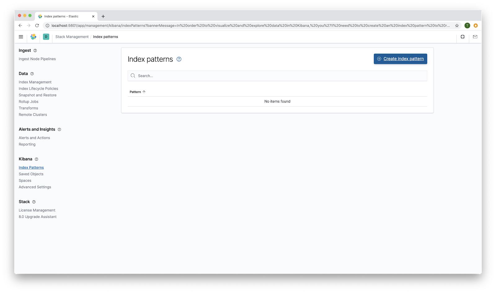
We can now take a look at our records. Go to `http://localhost:5601/app/discover#/`

You will need to do some setup to initialize index patterns. Click the Create index pattern button.

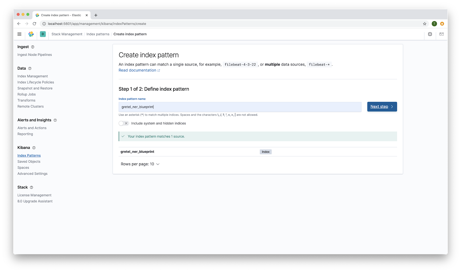
For step one, use gretel_ner_blueprint as the Index pattern name. Click Next step.

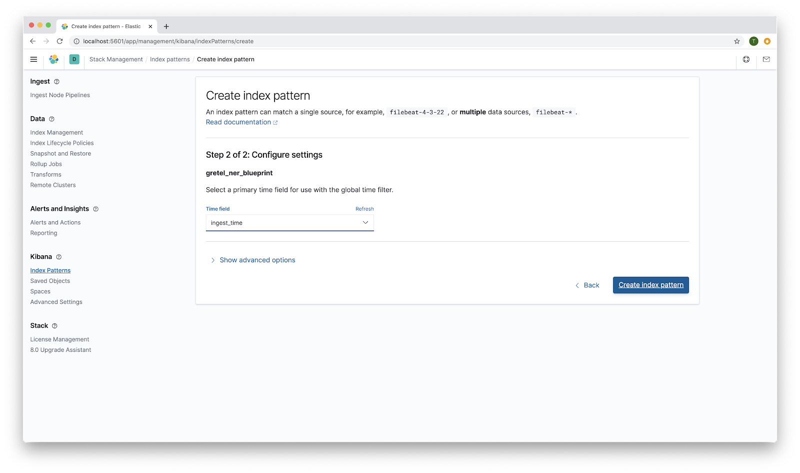
For Step 2, choose ingest_time as the primary time field for use with the global time filter. Because we loaded all of our records in one batch, this is not the most exciting time filter. If you have streaming data that you then index into Elasticsearch a time filter becomes more interesting and useful for detecting changing patterns in your data over time. Click Create index pattern.

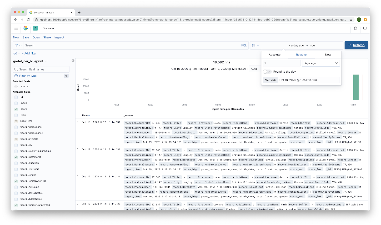
You will see a screen with a list of detected fields. Return to `http://localhost:5601/app/discover#/`. You may need to adjust the time range to see your records. Showing 1 day ago to present will suffice.

At this point you can do various queries within Kibana to filter results. As a somewhat contrived example, you can look for that rare Londoner who owns 3 or more cars and still needs to get a bike. Put record.NumberCarsOwned >= 3 and record.City: "London" into the search bar and hit the Refresh button. You should have a much smaller list of records.

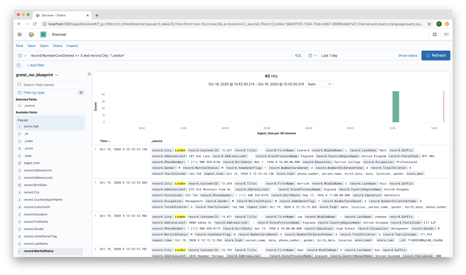
Clicking on one of the fields in the left hand column will expand it to show the counts for the top values for that field.

In addition to free form exploration, Kibana supports a rich set of dashboards. See the Kibana dashboard docs for getting started with this.

Viewing records programmatically

You can also make a raw query to pull back records if, for example, you need to generate regular reports from a script. Here is the same query (Londoners with 3 or more cars). We cap the number of records returned for space and clarity, but you can see the total number of records returned. We add an aggregation showing the breakdown of the number of children across the results, mimicking the bucketing shown on the left hand side of the discover view in Kibana.

As a slight twist, we also specify that we only want records that have the NER tag "location." In this data set, the records are homogeneous enough that this doesn't affect the results. If there were a tag that you expected to see infrequently, this would help catch those rare events.  A classic example of this is the "Thank you" note in a gift order that contains an SSN.

Note that if you try to use the score_high field for aggregations you will get an error! Because we have not specified an explicit type mapping up front, the field is typed as "text." You can specify "fielddata": "true" as part of the mapping for this field to make it available for aggregations. See this documentation for details on aggregations and this documentation for details on the text type.  Here is the query we use in the blueprint:

# Find records tagged with the NER 'location' label.  They must also be in London with 3 or more cars.
# Include an aggregation showing the number of children.
aggregation_query = {
    "query": {
        "bool": {
            "must": [
                {"match": {"record.City": "London"}}, 
                {"range": {"record.NumberCarsOwned": {"gte": 3}}},
                {"match": {"score_high": "location"}}
            ]
        }
    },
    "size": 3,
    "aggs" : {
        "children": {
            "terms": {"field": "record.TotalChildren"}
        }
    }
}

es.search(index=index_name, body=aggregation_query)

Conclusion

Elasticsearch and Kibana provide industry standard tools for the flexible exploration of data.  Combined with Gretel's NER analysis, users have a powerful and simple means to monitor trends in their data over time or spot suspicious outliers.